This document was originally a collection of blog posts with thousands of views on Medium, but honestly Medium doesn’t deserve them (clickbait eats quality there, and the whims of their editors). You’ll get an introduction to reinforcement learning how I learned to teach them at UC Berkeley for CS 188: Intro to Artificial Intelligence. I take a big detour into linear algebra to help ground some of the material in a field with a wider application base.

Brief History

Reinforcement learning holds its roots in the history of optimal control. The story began in the 1950s with exact dynamic programming, which broadly speaking is the structured approach of breaking down a confined problem into smaller, solvable sub-problems wikipedia, credited to Richard Bellman. Good history to know is that Claude Shannon and Richard Bellman revolutionized many computational sciences in the 1950s and 1960s.

Through the 1980s, some initial work on the link between RL and control emerged, and the first notable result was the Backgammon programs of Tesauro based on temporal-difference models in 1992. Through the 1990s, more analysis of algorithms emerged and leaned towards what we now call RL. A seminal paper is “Simple Statistical Gradient-Following Algorithms for Connectionist Reinforcement Learning” from Ronald J. Williams, which introduced what is now vanilla policy gradient. Note that in the title he included the term ‘Connectionist’ to describe RL — this was his way of specifying his algorithm towards models following the design of human cognition. These are now called neural networks, but just two and a half decades ago was a small subfield of investigation.

It was not until the mid-2000s, with the advent of big data and the computation revolution that RL turned to be neural network based, with many gradient based convergence algorithms. Modern RL is often separated into two flavors, being model “free” and model “based” RL, if you’re here for that, scroll to the end.

Markov Decision Processes (MDPs)

We start here because we need to learn about the model that is used to describe the world in most reinforcement learning problems.

Why should I care?

Anyone interested in the growth of reinforcement learning should know the model they’re built on — Markov Decision Processes. They set up the structure of a world with uncertainty in where actions will take you, and agents need to learn how to act.

Non-Deterministic Search

Search is a central problem to artificial intelligence and intelligent agents. By planning into the future, search allows agents to solve games and logistical problems — but they rely on knowing where a certain action will take you. In traditional, tree-based methods, an action takes you to a next state, there is no distribution of next-states. That means, if you have the storage for it, you can plan set, deterministic trajectories into the future. Markov Decision Processes make this planning stochastic, or non-deterministic. The list of topics in search related to this article is long — graph search, game trees, alpha-beta pruning, minimax search, expectimax search, etc.

In the real world, this is a far better model for how agents act. Every simple action we take — pouring the coffee, sending a letter, moving a joint — has an expected outcome, but there is a sort of randomness to life. Markov Decision Processes are the tool that makes planning capture this uncertainty.

What is Markov about MDPs?

Markov is all about Andrey Markov — a famous Russian mathematician most known for his work on stochastic processes.

“Markov” generally means that given the present state, the future and the past are independent.

Andrey Markov (1856–1922)

The key idea of making a Markovian system is memorylessness. Memorylessness is the idea that the history of a system does not impact the current state. In probability notation, memorylessness translates into this. Consider a sequence of actions yields a trajectory, and we are looking to see where the current action will take us. The long conditional probability could look like:

Now — if the system is Markovian, the history is all encompassed in the current state. So, our one step distribution is far simpler. This one step is a game-changer for computational efficiency. The Markov Property underpins the existence and success of all modern reinforcement learning algorithms.

Markov Decision Process (MDPs)

An MDP is defined by the following quantities:

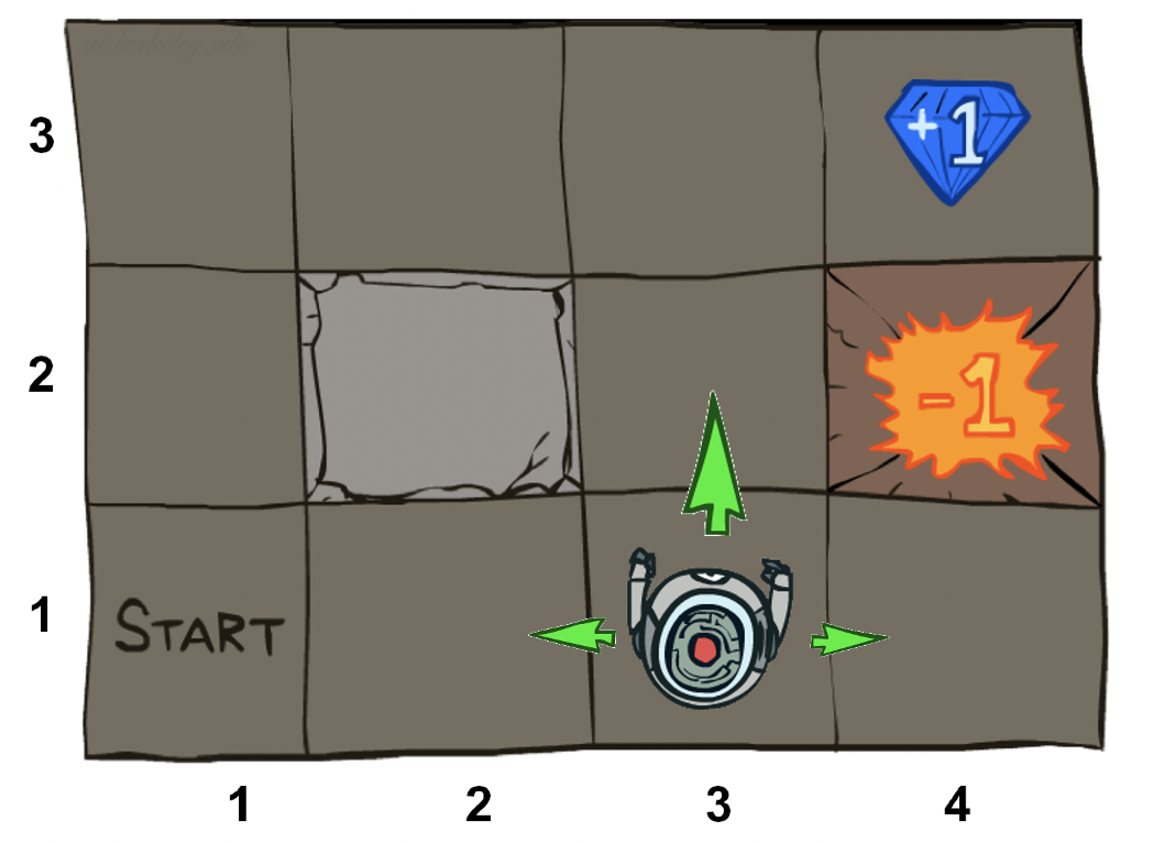
• Set of states s ∈ S. The states represent all the possible configurations of the world. In the example below, it is robot locations.
• Set of actions a ∈ A. The actions are the collection of all possible motions an agent can take. Below the actions are North, East, South, West.
• A transition function T(s,a,s’). T(s,a,s’) holds the uncertainty of an MDP. Given a current position, and a provided action, T governs how frequently a certain next state follows. In the example below, the transition function could be that the next state is in the direction of the action 80% of the time, but is off by 90degrees the other 20%. How does this affect planning? In the example below, the robot chose North, but there’s a 10% chance each of it going East or West.
• A reward function R(s,a,s’). Maximizing the sum of rewards is the goal of any agent. This function says how much reward is gained at each step. In general, there will be a small negative reward (cost) at each step to encourage fast solutions, and big positive (goal) or negative (failed task) rewards at terminal states. Below, the Gem and the Fire Pit are the terminal states.
• A start state s0, and maybe a terminal state.

What does this give us?

This definition gives us a finite world, we a set forward dynamics model. We know the exact probabilities for each transition, and how good each action is. Ultimately, this model is a scenario — a scenario where we will plan how to act knowing that our actions may go slightly awry.

If the robot is next to the fire pit, should the robot always choose North knowing that there’s a chance that North will send it East?

No — the optimal policy will be West. Going into the wall will eventually (20% chance) go North, and put the robot on track for the goal.

Policies

Learning how to act in an unknown environment is the final goal of understanding an environment. In MDPs, this is called the policy.

A policy is a function that gives you an action from a state. π*: S → A.

There are many methods of getting to a policy, but the core ideas are value and policy iteration. Both of these methods iteratively build estimates for the total utility of a state, and maybe an action.

The Utility of a state is the sum of (discounted) rewards.

Once every state has a utility, planning and policy generation at a high level becomes following the line of maximum utility. In MDPs and other learning approaches, the models add a discount factor γ to prioritize near term to long term rewards. The discount factor makes sense intuitively — humans and biological creates value money (or food) in hand now more than later. The discount factor also carries with it immense computational convergence help by changing the sum’s of rewards into a geometric series.

The hidden linear algebra of RL

How do fundamentals of linear algebra support what is going on in MDPs. This section is something you won’t get in a normal intro course, but I find it fun to consider the iterative updates when solving Markov Decision Process as a dynamical system.

Intro

How do fundamentals of linear algebra support the pinnacles of deep reinforcement learning? The answer is in the iterative updates when solving Markov Decision Process.

Reinforcement learning (RL) is the set of intelligent methods for iteratively learning a set of tasks. As computer science is a computational field, this learning takes place on vectors of states, actions, etc. and on matrices of dynamics or transitions. The states and vectors can take different forms, but how can we look at the convergence of the algorithms making headlines around the technology community? When we think of passing a vector of variables through some linear system, and getting a similar output, eigenvalues should come to mind.

Important values

There are two important characteristic utilities of a MDP — values of a state, and q-values of a chance node.

• Value of a state: The value of a state is the optimal recursive sum of rewards starting from a state. The value of the state to the left would be greatly different if the robot is in a fire pit, near a gem, or on a couch.
• Q-value of a state, action pair: The q-value is the optimal sum of discounted rewards associated with a state-action pair. The q-value of a state is determined by an action — so the q-values on the ledge will vary greatly if pointing in or out of flames!

These two values are related by mutual recursion, and Bellman updates.

Bellman Updates

Richard E. Bellman was a mathematician that laid the groundwork for modern control and optimization theory. Through a recursive one-step equation, a Bellman Update Equation, large optimization problems can be solved efficiently. With a recursive Bellman update, one can set up an optimization or control problem with Dynamic Programming, which is a process of creating smaller, more computationally tractable problems. This process proceeds recursively from the end — a receding horizon approach.

Richard E. Bellman (1920–1984) — Wikipedia.

1. Bellman Equation: Necessary condition for optimality in optimization problems formulated as Dynamic Programming.
2. Dynamic Programing: Process to simplify an optimization problem by breaking it down into an optimal substructure.

In reinforcement learning, we use the Bellman Update process to solve for the optimal values and q-values of a state-action space. This is ultimately formulating the expected sum of future rewards from a given location.

Here, we can see all of the values from the review interleaving. The notation (*)denotes optimal, so true or converged. We have the value of the state being determined by the best action, and a q-state, then two recursive definitions. The recursive values balance the probability of visiting any state in T(s,a,s’) and the reward of any transition R(s,a,s’) to create a global map for values of the state-action space.

The best value is tied to the best action-conditions q-value. Then the value and q-value update rules are very similar (weighting transitions, rewards, and discount). top) coupling of values to q-values; mid) Q-value recursion, bot) Value iteration. Source cs188 at UC Berkeley.

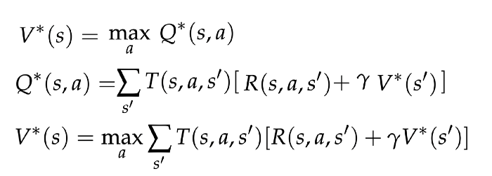
They key point here is that we are multiplying matrices (R, T), by vectors (V,U), to iteratively solve for convergence. The values will converge from any initial state because of how the values for one state are determined by their neighbors s’.

Reinforcement Learning?

“I was told there would be RL,” — you, reader, 8 minutes in. This is all reinforcement learning, and I assert understanding the assumptions and the model that the algorithms are built on will prepare you vastly better then just copying python tutorials from OpenAI. Do that after. I’ve mentored multiple students into working in RL, and the ones who get more done are always the ones that learn what is going on, and then how to apply it.

That being said, this is one small step away from online q-learning, where we estimate the same Bellman updates with samples of T and R rather than explicitly using them in the equations. All the same assertions apply, but it is over probability distributions and expectations. Q-learning is the famous algorithm that solved Atari games and more in 2015.

Hidden Math

Eigenvalues? Huh.

Recall an eigenvalue-eigenvector pair (λ, u) of a system A is a vector and scalar such that the vector acted on by the system returns a scalar multiple of the original vector.

The eigenvalue, eigenvector equation.

The beautiful thing about eigenvalues and eigenvectors is that when they span the state space (which they are guaranteed to do for most physical systems by something called generalized eigenvectors), every vector can be written as a combination of the other eigenvectors. Then, in discrete systems Eigenvectors control the evolutions from any initial state — any initial vector will combine to a linear combination of the eigenvectors.

Stochastic Matrices and Markov Chains

MDPs are very close to, but not the same in structure to Markov Chains. Markov chains are determined by transition matrix P. The probability matrix acts like the transition matrix T(s,a,s’) summed over the actions. In Markov Chains, the next state is determined by:

Evolution of a stochastic matrix.

This matrix P has some special values — you can see that this is an eigenvalue equation with all the eigenvalues equal to one (picture a λ=1 pre-multiplying the left side of the equation). In order to get a matrix guaranteed to have eigenvalues equal to one, all the columns must sum up to 1.

What we are looking for in RL now, is how does the evolution of our solutions relate to convergence of probability distributions? We do this by formulating the iterative operators for V* and Q* as a linear operator (a Matrix) B. Convergence can be tricky — the value and q-value vectors we use are not the eigenvectors — they converge to the eigenvectors, but that’s not important to seeing how eigenvectors govern the system.

The Bellman operator, B, like a linear transformation with eigenvector, eigenvalue pair of λ=1.

Any initial value distribution will converge to the shape of the eigenspace. This illustration doesn’t show the exact eigenvalues of the Bellman update, but how the shape of the space could evolve as the values recursively update. Initially, the values will be totally unknown, but as learning emerges — the known values will converge to match the environment exactly.

Bellman Updates to Matrices

So far, we know that if we can formulate our Bellman updates (which are linear updates) in a simpler form, a convenient eigen-structure will emerge. How can we formulate our Q update as a simple update equation? We start with a Q-iteration equation (Optimal value substituted for the equivalent Q-value equation on the right).

There’s a couple minor steps (and admittedly a couple big assumptions) that are needed to make this transition.

Moving our system towards a linear operator (Matrix)

i) Let us rephrase a couple of the terms to general forms

The first half of the update, the summation over R, T, is an explicit reward number; we call it R(s). Next, we change our summation over transitions to a probability matrix (matching a Markov matrix, convenient). Also, this leads into the next step — changing from Q to utilities. (Recall, you can take a maximization out of a sum (think of it as a more general upper bound).

Close to the Bellman matrix we want, where the P(s’|s,a) would dictate the evolution of our matrix.

ii) Let’s make this a vector equation

We are most interested in how the utility, U, evolves for a MDP. That utility implies the value or q-value. We simply can re-write our Q into a U without much of a change, but that means we are assuming a fixed policy.

Transforming the q-state to a general utility vector for eigenvalues.

It’s important to recall that even for a multi-dimensional, physical system —the utilities of a state are a vector if we stack all of the measured states into a long array. A fixed policy doesn’t change convergence — it just means we have to revisit this to learn how to get a policy iteratively.

iii) Assume a fixed policy

If you assume a fixed policy, the maximization over a disappears. The maximization operator is distinctly nonlinear, but there are forms in linear algebra that are eigenvectors plus an additional vector (hint — generalized eigenvectors).

This equation above is a general form of a Bellman update on Utility. We wanted a linear operator, B, then we could see how this is an eigenvalue evolution equation. It looks a little different, but this is ultimately the form we want, minus a couple linear algebra assertions, so we have our Bellman update.

The Bellman operator, B, like a linear transformation with eigenvector, eigenvalue pair of λ=1.

Computationally, one can get the eigenvectors we want, but doing so analytically is challenging because of the assumptions made along the way.

Takeaway

Linear operators show you how certain discrete, linear systems will evolve — and the environments we use in reinforcement learning follow that structure.

Eigenvalues and Eigenvectors of our collected data can represent the latent value space of a RL problem.

The nitty gritty of change of variables, linear transformations, fitting this into online q-learning (rather than the q-iteration here), and more will be in a future post.

Fundamental Methods of RL & MDPs

This section focuses on taking an understanding of basic MDPs and applying it to how it relates to a fundamental reinforcement learning method. The methods I will focus on are Value Iteration and Policy Iteration. These two methods underpin Q-value Iteration, which directly leads to Q-Learning.

Q-Learning kick-started the deep reinforcement learning wave we are on, so it is a crucial peg in the reinforcement learning student’s playbook.

Review Markov Decision Processes

Markov Decision Processes (MDPs) are the stochastic model underpinning reinforcement learning (RL). If you’re familiar, you can skip this section, but I added explanations for why each element matters in a reinforcement learning context.

Revisiting Definitions & RL

• Set of states s ∈ S, actions a ∈ A. The states and actions are the collection of all possible positions and motions of an agent. In advanced reinforcement learning, the states and actions often become continuous, which requires a rethink of our algorithms.
• A transition function T(s,a,s’). Given a current position, and a provided action, T governs how frequently a certain next state follows. In reinforcement learning, we no longer have access to this function, so the methods attempt to approximate it or learn implicit on sampled data.
• A reward function R(s,a,s’). This function says how much reward is gained at each step. In reinforcement learning, we no longer have access to this function, so we learn from sampled values r that lead the algorithms to explore environments and then exploit optimal trajectories.
• A discount factor γ (gamma) in [0,1] which tunes the value of immediate (next step) to future rewards. In reinforcement learning, we no longer have access to this function, γ (gamma) controls the convergence of most all learning algorithms and planning-optimizers through Bellman-like updates.
• A start state s0, and maybe a terminal state.

Leading towards reinforcement learning

Value Iteration

Learn the values for all states, then we can act according to the gradient. Value iteration learns the value of the states from the Bellman Update directly. The Bellman Update is guaranteed to converge to optimal values, under some non-restrictive conditions.

Learning a policy may be more direct than learning a value. Learning a value may take an infinite amount of time to converge to numerical precision of a 64bit float (think about a moving average averaging in a constant at every iteration, after starting with an estimate of 0, it will add a smaller and smaller nonzero number forever).

Policy Iteration

Learn a policy in tandem to the values. Policy learning incrementally looks at the current values and extracts a policy. Because the action space is finite, the hope is that it can converge faster than Value Iteration. Conceptually, the last change to the actions will happen well before the small rolling-average updates end. There are two steps to Policy Iteration.

The first is called Policy Extraction, which is how you go from a value to a policy — by taking the policy that maximizes over expected values.

The second step is Policy Evaluation. Policy evaluation takes a policy and runs value iteration conditioned on a policy. The samples are forever tied to the policy, but we know we have to run the iterative algorithms for way fewer steps to extract the relevant action information.

Policy evaluation step.

Like value iteration, policy iteration is guaranteed to converge for most reasonable MDPs because of the underlying Bellman Update.

Q-value Iteration

The problem with knowing optimal values is that it can be hard to distill a policy from it. The argmax operator is distinctly nonlinear and difficult to optimize over, so Q-value Iteration takes a step towards direct policy extraction. The optimal policy at each state is simply the max q-value at that state.

The reason most instruction starts with Value Iteration is that it slots into the Bellman updates a little more naturally. Q-value Iteration requires the substitution of two of the key MDP value relations together. After doing so, it is one step removed from Q-learning, which we will get to know.

Iterative algorithms?

Let’s make sure you understand all the terms. Essentially, each update is made up of two terms after the summation (and potentially a max term that selects an action). Let’s factor out the brackets and discuss how they relate to an MDP.

‍

The first term is a summation over the product T(s,a,s’)R(s,a,s’). This term represents the latent value and likelihood of a given state and transition. The T term, or transition, governs how likely it is to get a given reward from a transition (recall, a tuple s,a,s’determines a tuple where an action a takes an agent from state s to state s’). This will do things like weight low probability states with high rewards against frequent states with lower rewards.

The next term governs the “Bellman-ness” of these algorithms. It is a weighting of the data at the last step of the iterative algorithm — V, with the term above. This pulls information from neighboring states about value so that we can understand longer-term transitions. Think of this term as to where most of the recursive update happens, and the first term is a weighing prior determined by the environment.

Conditions on convergence

All of the iterative algorithms are told to “converge to the optimal value or policy, under some conditions.” What are those conditions you ask?

1. Total state-space coverage. The condition is that all state, action, next_state tuples are reached under the conditioned policy. Without this, some information from the MDP will be lost and Values can be stuck at the initial value.
2. Discount factor γ <1. This is because the Values for any loop that can be repeated can and will go to infinity.

Thankfully, in practice, these conditions are easy to meet. Most exploration has an epsilon-greediness that includes a chance at a random action, always (so any action is feasible) and a non-one discount factor results in more favorable performance. Ultimately, these algorithms work in plenty of settings, so they’re definitely worth giving a shot.

Reinforcement Learning

How do we make what we have seen into a reinforcement learning problem? We need to use samples rather than the true T(s,a,s’) and R(s,a,s’) functions.

Sample-based learning — how to solve a hidden MDP

The only difference between iterative methods in MDPs and the basic methods of solving a reinforcement learning problem is that RL samples from the underlying transition and reward functions of an MDP, rather than having it in the update rule. There are two things we need to update to get going, a replacement for T(s,a,s’)and a replacement for R(s,a,s’).

First, let us approximate the transition function as the average action conditioned transition for each observed tuple. All the values we have not seen are initialized with random values. This is the simplest form of model-based reinforcement learning (my research area).

(Above:An approximation for the transition function. The groundwork for advanced model-based reinforcement learning research.)

Now, all that is left is remembering what to do with the reward, right? But, we actually have a reward with each step, so we can get away with it (methods average out to the correct value with many samples). Consider approximating the Q-value iteration equation with a sampled reward, as below.

Sample-based Q-learning (actual RL).

End note on Q-learning

The above equation is Q-learning. We start with some vector Q(s,a) that is filled with random values, and then we collect interactions with the world and tune alpha. Alpha is a learning rate, so we will lower it when we think our algorithm is converging.

It works out that Q-learning converges really similarly to Q-value Iteration, but we are just running the algorithm with an incomplete view of the world.

The Q-learning used in robotics and games is in more complex feature spaces with neural networks approximating a large table of all the state-action pairs. For a summary of how Deep Q-Learning shocked the world, here is a great video until I write my own piece about it! But, how do these converge?

Convergence of Iterative Algorithms

Are there any simple bounds one can put on the rate of learning a task? A study in the context of Q-learning.

Deep reinforcement learning algorithms may be the most difficult algorithms in recent machine learning developments to put numerical bounds on their performance (among those that function). The reasoning is twofold:

1. Deep neural networks are nebulous black boxes, and no one truly understands how or why they converge so well.
2. Reinforcement learning task convergence is historically unstable because of the sparse reward observed from the environment (and the difficulty of the underlying task — learn from scratch!).

Here, I will walk you through a heuristic we can use to describe how RL algorithms can converge, and explain how to generalize it to more scenarios.

Generalizing the iterative updates

In the first section of new content I will recall the RL concepts I am using, and highlight the mathematical transformations needed to get a system of equations that evolves in discrete steps and has a convergence bound. This section follows closely from the linear algebra section earlier.

Reinforcement Learning

RL is the paradigm where we are trying to “solve” and MDP, but we don’t know the underlying environment. The simple RL solutions are sampling-based variants of fundamental MDP-solving algorithms (Value and Policy Iteration). Recall Q-value Iteration, which is the Bellman Update I will focus on:

Looking at how accurate Value Iteration or Policy Iteration distills to comparing a value vector after each assignment (←) in the above equation, which is one round of the recursive update. The convergence of these methods yields a measure proportional to how reinforcement learning algorithms will converge because reinforcement learning algorithms are sampling-based versions of Value and Policy Iteration, with a few more moving parts.

Recall: Q-learning is the same update rule as Q-value Iteration, but the transition function is replaced by the action of sampling and the reward function is replaced with the actual sample, r, received from the environment.

Linear Operator and Eigenvectors

We need to formulate our Bellman Updates as a linear operator, B,(a matrix is a subset of linear operators) and see if we can get it to behave as a stochastic matrix. A stochastic matrix is guaranteed to have an eigenvector paired with the eigenvalue 1.

This says, we can study the iterative updates in RL like we would the evolution of an eigenspace where lambda is 1.

For now, we need to make a couple of notational changes to transition from formulas on Q-values in a matrix to formulas that are acting on Utilities in a vector (Utilities generalize to values and Q-values, anyways because it is defined as the discounted sum of rewards).

1. We know utilities are proportional to q-values; change the notation. We will use U(s).
2. Rearranging the utilities as a vector is like the flatten() function of many coding libraries (e.g. shifting an XY state-space to a 1d vector indexing across the states). We get u‍

‍

Transforming the q-state to a general utility vector for eigenvalues. These changes are crucial for formulating the problem as eigenvectors.

Understanding the Pieces of Q-learning

Start with the base equation for Q-value iteration below, how can we generalize this to a linear system? Recall the assumptions we made in the linear algebra section: 1) that we can average over the transition and reward distributions to make that a static vector R(s) and 2) the term with the Q values and the transition probabilities is like a stochastic matrix.

This leaves us with a final form (merging equations from this section, and the end of the eigenvalue section). Can we use this as the linear operator that we need? Consider if we are using the optimal policy (without loss of generality), then the tricky maximum over actions drops out, leaving us with:

And, re-writing like a generalized eigenvector, we get:

This is as closer as we can get to making this a pure eigenvector equation. It’s very close to what is called a generalized eigenvector.

Studying Convergence

In this section, I will derive a relationship that guarantees a minimum error of epsilon after N steps and show what it means.

The system we can study

We saw above that we can formulate the utility update rule in a way that is very close to an eigenvector, but we were off by a constant vector r representing the underlying reward surface of an MDP. What happens if we take the difference between two utility vectors? The constant term drops out.

Taking the difference between two utility vectors, we see that the r vector can cancel out.I

We now have our system that we can study like a dynamical system of eigenvectors, but we are working in the space of the difference between utilities, with a matrix B —the sum of weighted transition probabilities. Because the utility vectors are defined by each other, we can magically rearrange this (substitute the recursive Bellman Equation, take the norm). The error after a Bellman update is reduced by the discount factor.

Studying the difference between any utility estimate is ingenious, because it shows a) how an estimate differs from the true or b) how the data from only the recursive update evolves (not the little vector r).

An epsilon-N Relation

Any convergence proof will be looking for a relationship between the error bound, ε, and the number of steps, N,(iterations). This relationship will give us the chance to bound the performance with an analytical equation.

We want the bound of our Utility error at step N — b(N) — to be less than epsilon. The bound will be an analytical expression, and epsilon is a scalar representing the norm of the difference between the estimated and true utility vectors.

In other words, we are looking for a bound for epsilon that this a function of N.

To start, we know (by definition of an MDP) that the reward at each step, r, is bounded in the interval [-Rmax, +Rmax]. Then, looking at the definition of utility (discounted sum of reward) as a geometric series, we can bound the difference from any vector to the true vector. (Proof for geometric series convergence).

First, recall the definition of utility: The expected sum of discounted reward.

Next, our starting point for convergence. Consider the difference between the true utility U and the initial utility U(0) from the convergence of a geometric series.

The bound comes from the worst-case estimate — where the true reward at every step is +Rmax, but we initialize our estimate to -Rmax. Alas, we have an initial bound on the error of our utilities! Recall U0 is what we initialize the utility vector to, and then the index will increase each time we run a Bellman Update.

To the Bellman Updates — how does this bound at initialization evolve with each step? Above, we see that the error is reduced by the discount factor at each step(from how the sum in the recursive update is always prepended with a gamma). This evolves below into a series of decreasing errors with each iteration.

The convergence of the difference between the current Utility update (U_i) and the true value U.

All that is left is declaring the bound, epsilon, in relation to the number of steps, N.

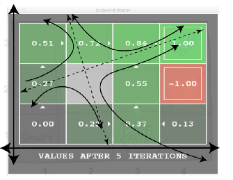
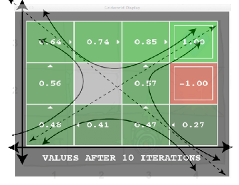
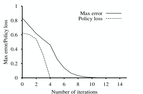
The Outcome — Visualizing Convergence

On the right-hand side of the equation above, we have a bound on the accuracy of our utility estimate.

Logically — for any epsilon, we know that the error will be less than epsilon in N steps.

We can also change back and forth between epsilon and N with a mathematical trick — so if we know how accurate we want the estimates to be, we can solve for how long to let our algorithm run!

By taking the logarithm of both sides we can solve for the number of iterations to reach said bound!

The bound we have found is the bound on the cumulative value error across the state-space (solid line below). What the astute reader will wonder is, how does the policy error compare? Conceptually, this means, ‘in how many states would the current policy differ from the optimal?’ Turns out, with some normalization of the values (so they are numerically similar in magnitude) the policy error converges faster and gets to zero more rapidly (no asymptote!).

This represents the advantage in some situations to use Policy Iteration over Value Iteration. Does it carry to more algorithms?

Bounding Recent Deep RL Algorithms

Bounding deep RL algorithms is what everyone wants. We have seen impressive results in recent years where robots can run, fold towels, and playgames. It would be fantastic if we have bounds on performance.

What we can do, is bound how our representation of the world will converge. We have shown that the utility function will converge. There are two lasting challenges:

1. we are not given the reward function for real-life tasks, we must design it.
2. running these iterative algorithms is currently not safe. Robotic exploration involves a lot of force, interaction, and (realistically) damage.

We can study algorithm convergence, but the majority of engineering problems limiting adoption of deep RL for real world tasks are reward engineering and safe learning.

That is where I leave you — a call to action to help us engineer better systems, so we can show off more of the underlying mathematics governing it. There’s an explanation of recent algorithmic advances below, but the fundamental understanding of what RL is finishes here.

Gists of Some RL Algorithms (Sp 2019)

I conclude with a resource for getting the gist of RL algorithms without needing to surf through piles of documentation or equations.

A resource for getting the gist of RL algorithms without needing to surf through piles of documentation — a resource for students and researchers, without a single formula. As a reinforcement learning (RL) researcher I often need to remind myself of the subtle differences between the algorithms. Here I want to create a list of algorithms and a sentence or two for each that distinguishes it from others in its sub area. I pair this with a brief historical introduction to the field.

Model Free RL

Model free RL directly generates a policy for an actor. I like to think of it as end-to-end learning of how to act, with all the environmental knowledge being embedded in this policy.

Policy Gradients Algorithms

Policy gradient algorithms modify an agent’s policy to track those actions that bring it higher reward. This lends these algorithms to be on-policy, so they can only learn from actions taken within the algorithm.

Simple Statistical Gradient-Following Algorithms for Connectionist Reinforcement Learning (REINFORCE) — 1992: This paper kickstarted the policy gradient idea, suggesting the core idea of systematically increasing the likelihood of actions that yield high rewards.

Value Based Algorithms

Value based algorithms modify an agent’s policy based on the perceived value of a given state.This lends these algorithms to be off-policy because an agent can update its internal value structure of a state by reading the reward function from any policy.

Q-Learning — 1992: Q-learning is the classic value based method in modern RL, where the agent stores a perceived value for each action, state pair, which then informs the policy action.

Deep Q-Network (DQN) — 2015: Deep Q-Learning simply applies a neural network to approximate the Q function for each action and state, which can save vast amounts of computational resources, and potentially expand to continuous time action spaces.

Actor-Critic Algorithms

Actor-critic algorithms take policy based and value based methods together — by having separate network approximations for the value (critic) and actions (actor). These two networks work together to regularize each other and create, hopefully, more stable results. Summary of Actor Critic Algorithms: source— Arulkumaran et al. “A Brief Survey of Deep Reinforcement Learning.”

Actor Critic Algorithms — 2000: This paper introduced the idea of having two separate, but intertwined models for generating a control policy.

Moving on From the Basics

A decade later, we find ourselves in an explosion of deep RL algorithms. Note that in all the press you read, deep at the core is referring to methods using neural network approximations.

Policy gradient algorithms regularly suffer from noisy gradients. I talked about one change in the gradient calculations recently proposed in another post, and a bunch of the most recent ‘State of the Art’ algorithms at their time looked to address this, including TRPO and PPO.

Trust Region Policy Optimization (TRPO) — 2015: Building on the actor critic approach, the authors of TRPO looked to regularize the change in policies at each training iteration, and they introduce a hard constraint on the KL divergence1, or the information change in the new policy distribution. The use of a constraint, rather than a penalty, allows bigger training steps and faster convergence in practice.

Proximal Policy Optimization (PPO) — 2017: PPO builds on a similar idea as TRPO with the KL Divergence, and addresses the difficulty of implementing TRPO (which involves conjugate gradients to estimate the Fisher Information matrix), by using a surrogate loss function taking into account the KL divergence. PPO uses clipping to make this surrogate loss and assist convergence.

Deep Deterministic Policy Gradient (DDPG) — 2016: DDPG combines improvements in Q learning with a policy gradient update rule, which allowed application of Q learning to many continuous control environments.

Combining Improvements in Deep RL (Rainbow) — 2017: Rainbow combines and compares many innovations in improving deep Q learning (DQN). There are many papers referenced here, so it can be a great place to learn about progress on DQN:

• Prioritization DQN: Replay transitions in Q learning where there is more uncertainty, ie more to learn.
• Dueling DQN: Separately estimates state values and action advantages to help generalize actions.
• A3C: Learns from multi-step bootstraps to propagate new knowledge to earlier in the networks.
• Distributional DQN: Learns a distribution of rewards rather than just the means.
• Noisy DQN: Employs stochastic layers for exploration, which makes action choices less exploitative.

The next two incorporate similar changes to the actor critic algorithms. Note that SAC is not a successor to TD3 as they were released nearly concurrently, but SAC uses a few of the tricks also used in TD3.

Twin Delayed Deep Deterministic Policy Gradient (TD3) — 2018: TD3 builds on DDPG with 3 key changes: 1) “Twin”: learns two Q functions simultaneously, taking the lower value for the Bellman estimate to reduce variance, 2) “Delayed”: updates the policy less frequently than the Q function, 3) adds noise to the to the target action to lower exploitative policies.

Soft Actor Critic (SAC) — 2018: To use model-free RL in robotic experiment the authors looked to improve sample efficiency, the breadth of data collection, and safety of exploration. Using entropy based RL they control exploration along with DDPG style Q function approximation for continuous control. Note: SAC also implemented clipping like TD3, and using a stochastic policy it benefits from regularizing action choice, which is similar to smoothing.

Many people are very excited about the applications of model-free RL as sample complexity falls and results rise. Recent research has brought an increasing portion of these methods to physical experiments, which is bringing the prospects of widely available robots one step closer.

Model Based RL

Model based RL(MBRL) attempts to build knowledge of the environment, and leverages said knowledge to take an informed action. The goal of these methods is often to reduce sample complexity on the model-free variants that are closer to end-to-end learning.

Probabilistic Inference for Learning Control (PILCO) — 2011: This paper is one of the first in model-based RL, and it proposed a policy search method (essentially policy iteration) on top of a Gaussian Process (GP) dynamics model (built in uncertainty estimates). There have been many applications of learning with GPs, but not as many core algorithms to date.

Probabilistic Ensembles with Trajectory Sampling (PETS) — 2018: PETS combines three parts into one functional algorithm: 1) a dynamics model consisting of multiple randomly initialized neural networks (ensemble of models), 2) a particle based propagation algorithm, and 3) and simple model predictive controller. These three parts leverage deep learning of a dynamics model in a potentially generalizable fashion.

Model-Based Meta-Policy-Optimization (MB-MPO) — 2018: This paper uses meta-learning to choose which dynamics model in an ensemble best optimizes a policy and mitigate model bias. This meta-optimization allows MBRL to come closer to asymptotic model-free performance in substantially lower samples.

Model-Ensemble Trust Region Policy Optimization (ME-TRPO) — 2018: ME-TRPO is the application of TRPO on an ensemble of models assumed to be the ground truth of an environment. A subtle addition to the model-free version is a stop condition on policy training only when a user defined proportion of models in an ensemble no longer sees improvement when the policy is iterated.

Model-Based Reinforcement Learning for Atari (SimPLe) — 2019: SimPLe combines many tricks in the model-based RL area with a variational auto-encoder modeling dynamics from pixels. This shows the current state of the art for MBRL in Atari games (personally I think this is a very cool piece to read, and expect people to build on it soon).

The hype behind model-based RL has been increasing in recent years. It has often been given a short look because it lacks the asymptotic performance of its model-free counterparts. I am particularly interested in it because it has enabled many experiment only, exciting applications including: quadrotors and walking robots.

References and Resources:

A great review of deep RL as of 2017. And, these two:

CS 294-112 Berkeley Deep RL Course (now of a new name CS285…)

Spinning Up in Deep RL